RGB文件三通道分量熵计算

import matplotlib.pyplot as plt
import cv2 as cv
import numpy as np

eps = np.spacing(1)  # 浮点精度，用于防止log(0)

# 读取图像，转化为256*256*3
f = open("test.rgb", "rb")
data = f.read( )
f.close( )
data = [int(x) for x in data]
data = np.array(data).reshape((256, 256, 3)).astype(np.uint8)

# 绘制原图和三通道图像预览
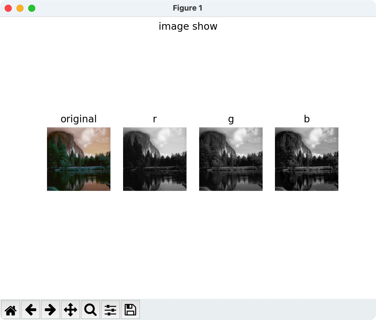
fig_img = plt.subplots(1, 4)
plt.subplot(1, 4, 1)
plt.imshow(data)
plt.title("original")
plt.axis('off')
plt.subplot(1, 4, 2)
plt.imshow(data[:, :, 0], cmap="gray")
plt.title("r")
plt.axis('off')
plt.subplot(1, 4, 3)
plt.imshow(data[:, :, 1], cmap="gray")
plt.title("g")
plt.axis('off')
plt.subplot(1, 4, 4)
plt.imshow(data[:, :, 2], cmap="gray")
plt.title("b")
plt.axis('off')
plt.suptitle('image show')
plt.show( )

# 绘制三通道直方图
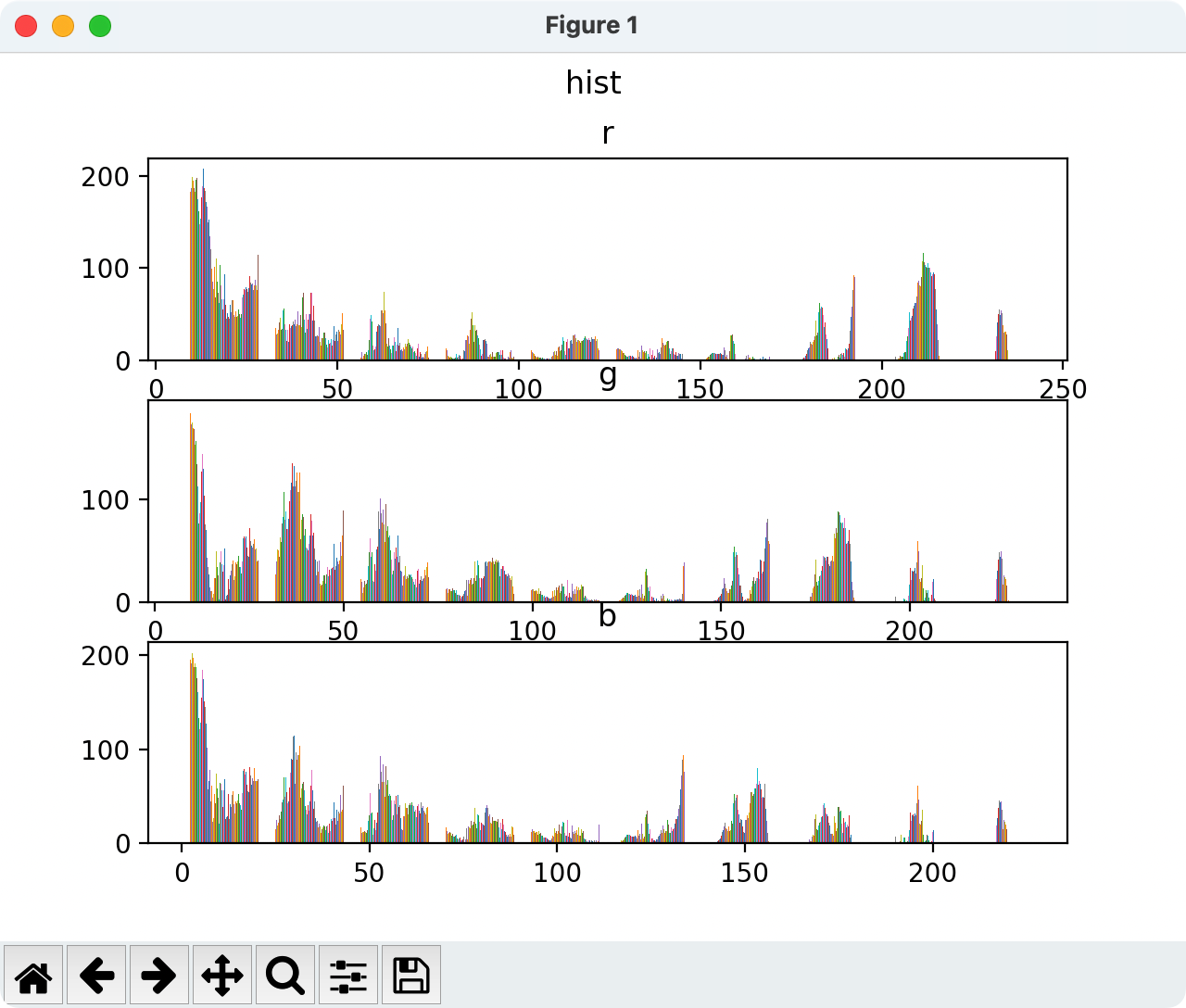
fig_hist = plt.subplots(3, 1)
plt.subplot(3, 1, 1)
plt.hist(data[:, :, 0])
plt.title('r')
plt.subplot(3, 1, 2)
plt.hist(data[:, :, 1])
plt.title('g')
plt.subplot(3, 1, 3)
plt.hist(data[:, :, 2])
plt.title('b')
plt.suptitle('hist')
plt.show( )

# 计算概率分布
p = np.zeros([3, 256])
for i in range(3):
    for j in range(256):
        for k in range(256):
            index = data[k][j][i]
            p[i][index] = p[i][index] + 1

# 计算熵
H = [0, 0, 0]
for i in range(3):
    tot = p[i].sum( )
    p[i] = p[i] / tot
    for j in range(256):
        H[i] = H[i] - p[i][j] * np.log2(p[i][j] + eps)
print(H)

[6.856861210882921, 7.178462484835032, 7.229552890551773]